X-Ray Chest Disease Detection with CNNs for Medical Imaging

Medical datasets are often imbalanced, where the number of samples in the disease class is much less than the number of samples in the normal class. This imbalance in the dataset can lead to a model that has poor predictive performance, specifically for the minority class, but can appear to be accurate.

This is extremely dangerous in the medical field, where a model that appears to be accurate but is not, can lead to misdiagnosis and death. We will discuss this in more detail later in the guide.

The dataset we will be using is the full NIH Chest X-ray dataset, which contains 112,120 X-ray images, where each image is labeled with up to 14 different diseases. The labels were created using Natural Language Processing (NLP) to mine the associated radiological reports. The labels are expected to be >90% accurate.

The code uses the whole dataset, which is about 45GB in size. We also used Data Augmentation for the underrepresented diseases, which added more images to the dataset. Caution: The code uses over 20GB of RAM, so make sure you have enough RAM before running it. I also recommend using a GPU for training as we will be training on about 83,000 images.

Disease Classes

There are 14 different diseases that we are trying to predict. The diseases are:

• Atelectasis: The partial or complete collapse of the lung, which is caused by a blockage of the air passages (bronchus or bronchioles) or by pressure on the lung.

• Consolidation: When the air that usually fills the small air-filled air pockets in the lung (alveoli) is replaced with blood, pus, water or something else.

• Infiltration: An infiltrate is substance denser than air, such as pus, blood, or protein, which lingers or spreads within the parenchyma (lung tissue) of the lungs.

• Pneumothorax: A collapsed lung that occurs when air leaks into the space between the lung and the chest wall, which puts pressure on the lung and causes it to collapse.

• Edema: A condition in which fluid builds up in the lungs. It is often caused by heart problems, but it can also occur from nonheart-related problems.

• Emphysema: A condition in which the air sacs (alveoli) of the lungs are gradually damaged and enlarged, causing breathlessness.

• Fibrosis: The thickening and scarring of connective tissue, causing difficulty of breathing.

• Effusion: An abnormal amount of fluid between the lungs and the chest wall.

• Pneumonia: An infection that affects one or both lungs, causing the air sacs of the lungs to fill up with fluid or pus.

• Pleural_Thickening: A condition in which the pleura (thin membrane that lines the lungs and chest wall) thickens.

• Cardiomegaly: A condition in which the heart is enlarged.

• Nodule: A small mass of rounded or irregular shape, smaller than 3cm in diameter.

• Hernia: A condition in which part of the lung tissue is pushed through a tear, or bulging through a weak spot, in the chest wall, neck passageway or diaphragm.

• Mass: A growth of tissue that is over 3cm in diameter.

Data Collection and Cleaning

Let’s start by importing the necessary libraries and setting up our environment:

# Import necessary libraries
import numpy as np
import pandas as pd
import matplotlib.pyplot as plt
import seaborn as sns
import tensorflow as tf
import os
from sklearn.model_selection import train_test_split
import glob
from sklearn.metrics import classification_report

# Set style and color palette
sns.set(style='darkgrid', palette='mako')

# Change the setting and put it in a dictionary
plot_settings = {
  'font.family': 'calibri',
  'axes.titlesize': 18,
  'axes.labelsize': 14,
  'figure.dpi': 140,
  'axes.titlepad': 15,
  'axes.labelpad': 15,
  'figure.titlesize': 24,
  'figure.titleweight': 'bold',
}

# Use the dictionary variable to update the settings using matplotlib
plt.rcParams.update(plot_settings)

# Check if the GPU is available
print("GPU is", "available" if tf.config.list_physical_devices('GPU') else "NOT AVAILABLE")

First, we’ll download the dataset using the Kaggle API and read the data entry CSV file:

# Download the dataset and unzip it
!kaggle datasets download -d nih-chest-xrays/data -p /data --unzip

# Read the data entry csv file, which contains the image file names and their corresponding labels
df = pd.read_csv('data/Data_Entry_2017.csv')

Next, we need to collect all the image paths from the dataset folders:

# Initialize an empty list to store the image paths
image_paths = []

# Loop over the range from 1 to 12
for i in range(1, 13):
  # Create a string with the folder name for each iteration
  folder_name = f'data/images_{i:03}'
  
  # Get all files in the current subfolder
  files_in_subfolder = glob.glob(f'{folder_name}/images/*')
  
  # Extend the list of image paths with the paths from the current subfolder
  image_paths.extend(files_in_subfolder)

# Check the length of the image paths list
print(f"Total number of images: {len(image_paths)}")

# Add the image paths to the dataframe
df['Image Path'] = image_paths

# Create a new dataframe to store the image paths, labels, and patient IDs
df = df[['Image Path', 'Finding Labels', 'Patient ID']]

Now that we have our image paths, we need to process the disease labels. We’ll create binary columns for each disease:

# Make a list of all the labels
diseases = ['Atelectasis', 'Cardiomegaly', 'Consolidation', 'Edema', 'Effusion', 'Emphysema',
          'Fibrosis', 'Hernia', 'Infiltration', 'Mass', 'Nodule', 'Pleural_Thickening',
          'Pneumonia', 'Pneumothorax']

# For each label, make a new column and
# assign 1 if the disease is present and 0 if the disease is absent
for disease in diseases:
  df[disease] = df['Finding Labels'].apply(lambda x: 1 if disease in x else 0)

Exploratory Data Analysis

Let’s analyze the distribution of diseases in our dataset:

# What are the label counts for each disease?
label_counts = df[diseases].sum().sort_values(ascending=False)

# Plot the value counts
plt.figure(figsize=(12, 8))
sns.barplot(x=label_counts.values, y=label_counts.index)
plt.xlabel('Number of Patients')
plt.ylabel('Disease')
plt.title('Number of Patients per Disease')
plt.show()

# Calculate percentage of each disease
unique_labels = df[diseases].sum().sort_values(ascending=False)

# Plot the percentage of each label
plt.figure(figsize=(12, 8))
sns.barplot(x=unique_labels.values / len(df) * 100, y=unique_labels.index)
plt.xlabel('Percentage')
plt.ylabel('Disease')
plt.title('Percentage of Each Disease')
plt.show()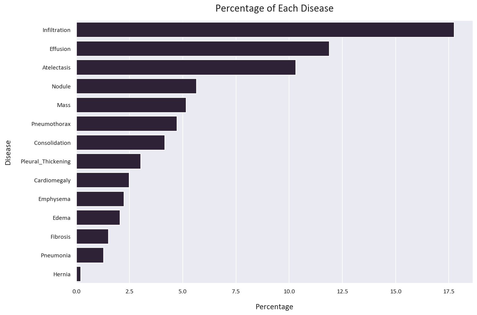

As we can notice, the data is extremely unbalanced towards the normal class. This is a common problem in medical datasets, where the number of positive samples is usually much smaller than the number of negative samples. This is a problem because most machine learning algorithms are designed to maximize accuracy and reduce error. Therefore, they tend to perform poorly on unbalanced datasets. In this case, the algorithm will tend to classify all samples as negative, resulting in a high apparent accuracy but poor performance in the positive class.

Let’s analyze how many diseases each patient has:

# How many diseases does each patient have?
label_counts = df[diseases].sum(axis=1).value_counts().sort_index()

# Plot the value counts
plt.figure(figsize=(12, 8))
sns.barplot(x=label_counts.index, y=label_counts.values)
plt.xlabel('Number of Diseases')
plt.ylabel('Number of Patients')
plt.title('Number of Diseases per Patient')
plt.show()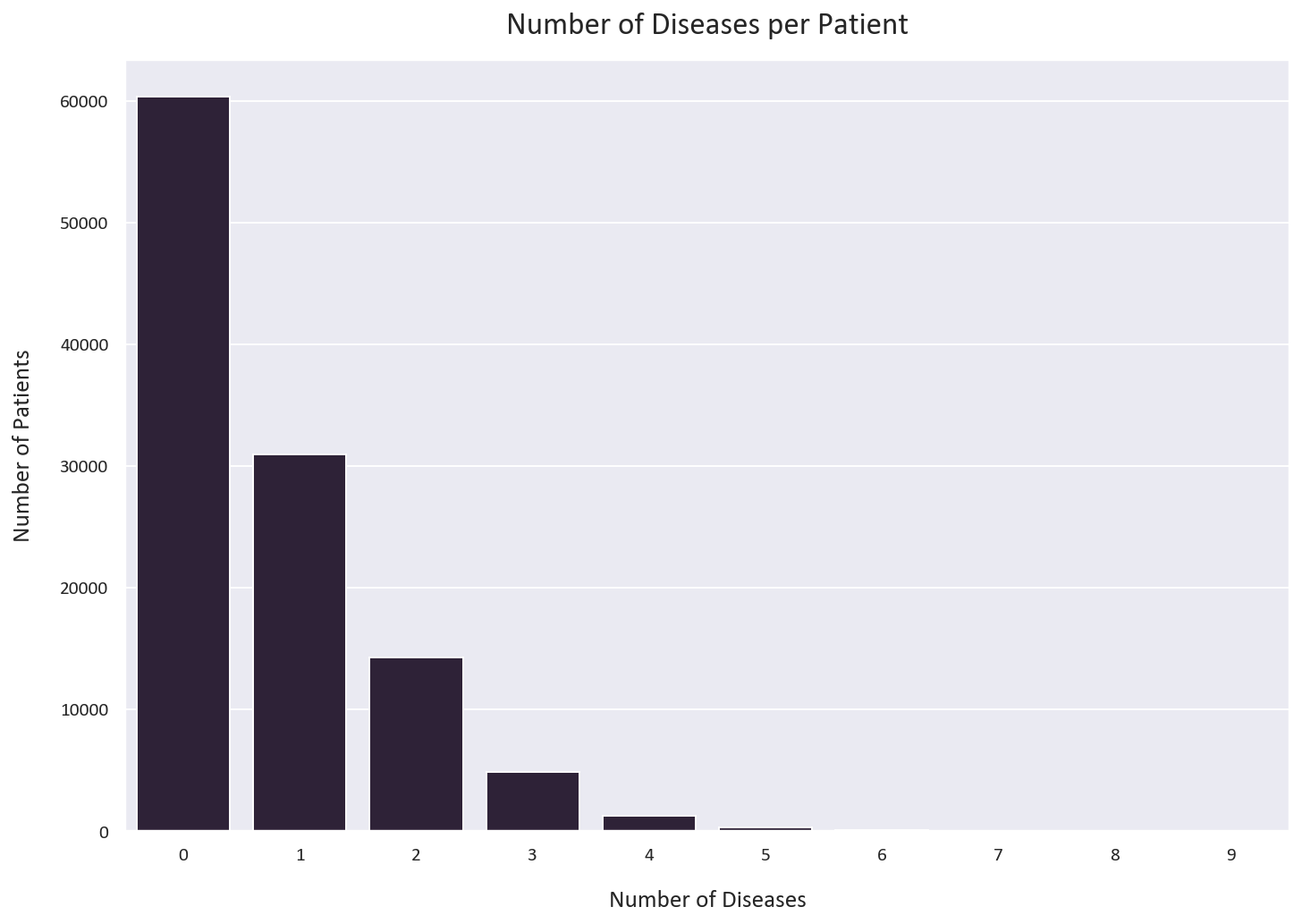

Let’s also visualize the positive and negative cases for each disease:

# Melt the dataframe to convert the diseases to rows
melted_df = pd.melt(df[diseases])

# Get the count of each disease
count_df = melted_df.groupby(['variable', 'value']).size().reset_index().rename(columns={0: 'count'})

# Calculate the total count for each 'variable'
total_count = count_df.groupby('variable')['count'].transform('sum')

# Calculate the percentage of each disease
count_df['Percentage'] = count_df['count'] / total_count * 100

# Plot the percentage of each disease
plt.figure(figsize=(12, 8))
sns.barplot(x='Percentage', y='variable', hue='value', data=count_df)
plt.xlabel('Percentage')
plt.ylabel('Disease')
plt.title('Positive and Negative Percentages of Each Disease')
plt.legend(labels=['Negative', 'Positive'])
plt.tight_layout()
plt.show()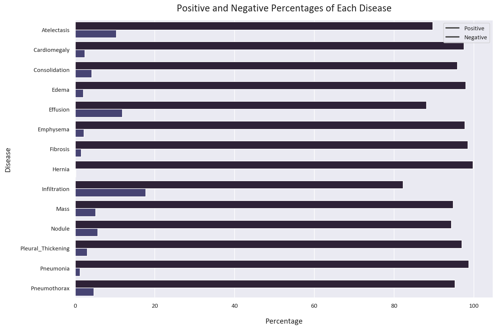

As we discussed earlier, the positive cases are much less than the negative cases. If a model is trained on this dataset, it will tend to classify most cases as negative, resulting in a high apparent accuracy. However, the model will perform poorly on the positive cases, which is dangerous in the medical field. This means that the model will tend to classify most patients as healthy, even if they have a disease. This can lead to misdiagnosis and death.

This is why we need to use other metrics to evaluate the performance of our model. In this case, we will use the AUC ROC, recall, and precision metrics.

• AUC ROC: The area under the Receiver Operating Characteristic curve. It is a probability curve that plots the True Positive Rate (TPR) against the False Positive Rate (FPR) at various threshold values and essentially separates the positive and negative cases. The higher the AUC, the better the model is at predicting positive and negative cases. This is a good metric to use for evaluating the performance of our model.

However, this metric alone could be deceiving. For example, if we have a dataset with 99% negative cases and 1% positive cases, a model that classifies all cases as negative will have a high AUC ROC. This is because the model will have a high True Negative Rate (TN) and a low False Positive Rate (FP). However, this model will perform poorly on the positive cases. This is why we need to use other metrics as well. This article explains this in more detail

• Precision: The number of true positives divided by the number of true positives and false positives. It is the ability of the classifier to not label a negative sample as positive. A high precision means that the classifier will not label a negative sample as positive very often. This will prevent false positives, where a patient is diagnosed with a disease when they do not have it. However, a high precision can lead to false negatives, where a patient is told they do not have a disease when they actually do. This is dangerous and can lead to misdiagnosis and death.

• Recall: The number of true positives divided by the number of true positives and false negatives. It is the ability of the classifier to find all positive samples. A high recall means that the classifier will not miss a positive sample very often. This will prevent false negatives, where a patient is told they do not have a disease when they actually do. However, a high recall can lead to false positives, where a patient is diagnosed with a disease when they do not have it. This is less dangerous than false negatives, as these patients are usually sent for further testing to confirm the diagnosis.

Data Quality and Preprocessing

When working with medical imaging datasets, several important considerations need to be addressed:

1. Image Quality: Medical images can vary significantly in quality due to:

   • Different imaging equipment and settings
   • Patient movement during image capture
   • Varying exposure levels
   • Presence of artifacts

2. Data Cleaning: Before processing, we should:

   • Remove corrupted or unreadable images
   • Check for and handle duplicate images
   • Verify label consistency
   • Ensure proper image orientation

3. Memory Management: Given the large dataset size (45GB), efficient data handling is crucial:

   • Use data generators to load images in batches
   • Process images on-the-fly when possible
   • Clear memory after processing each batch
   • Consider using memory-mapped files for large arrays

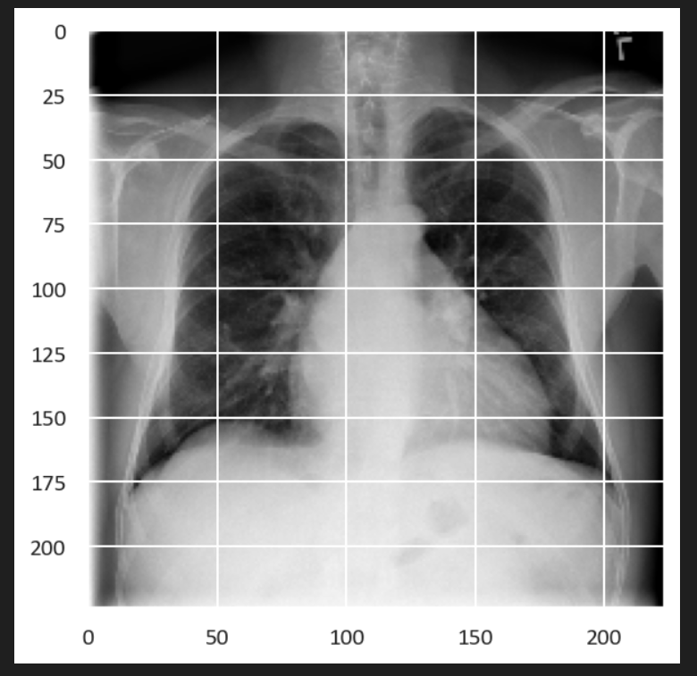
Let’s look at an example chest X-ray from our dataset:

Next, we have to deal with data leak, which is a very common problem in medical datasets. Data leak happens when the same patient is present in both the training and testing datasets. This is a problem because the model will learn to recognize the patient instead of the disease. This will result in high accuracy but poor performance in the real world.

In this case, we must make sure that the training, validation, and testing datasets are completely separated. We will use the patient ID to separate the datasets. We will first split the dataset into training and testing datasets. Then, we will split the training dataset into training and validation datasets. This will ensure that the same patient is not present in two different datasets.

Data Preprocessing and Data Augmentation

We will be using a 60/20/20 split for the training, validation, and testing datasets as we will be augmenting the training dataset.

# Define the image size and batch size
IMG_SIZE = [224, 224]
BATCH_SIZE = 32

# Get unique patient IDs
patient_ids = df['Patient ID'].unique()

# Split the patient IDs into train, validation, and test sets (60/20/20 split)
train_ids, test_ids = train_test_split(patient_ids, test_size=0.2, random_state=0)
train_ids, val_ids = train_test_split(train_ids, test_size=0.26, random_state=0) # 0.26 x 0.8 ~= 0.2

# Create dataframes for train, validation, and test sets
train_df = df[df['Patient ID'].isin(train_ids)]
val_df = df[df['Patient ID'].isin(val_ids)]
test_df = df[df['Patient ID'].isin(test_ids)]

# Drop the 'Patient ID' column
train_df = train_df.drop(['Patient ID', 'Finding Labels'], axis=1).reset_index(drop=True)
val_df = val_df.drop(['Patient ID', 'Finding Labels'], axis=1).reset_index(drop=True)
test_df = test_df.drop(['Patient ID', 'Finding Labels'], axis=1).reset_index(drop=True)

Let’s check if the distribution of the classes is similar in all datasets:

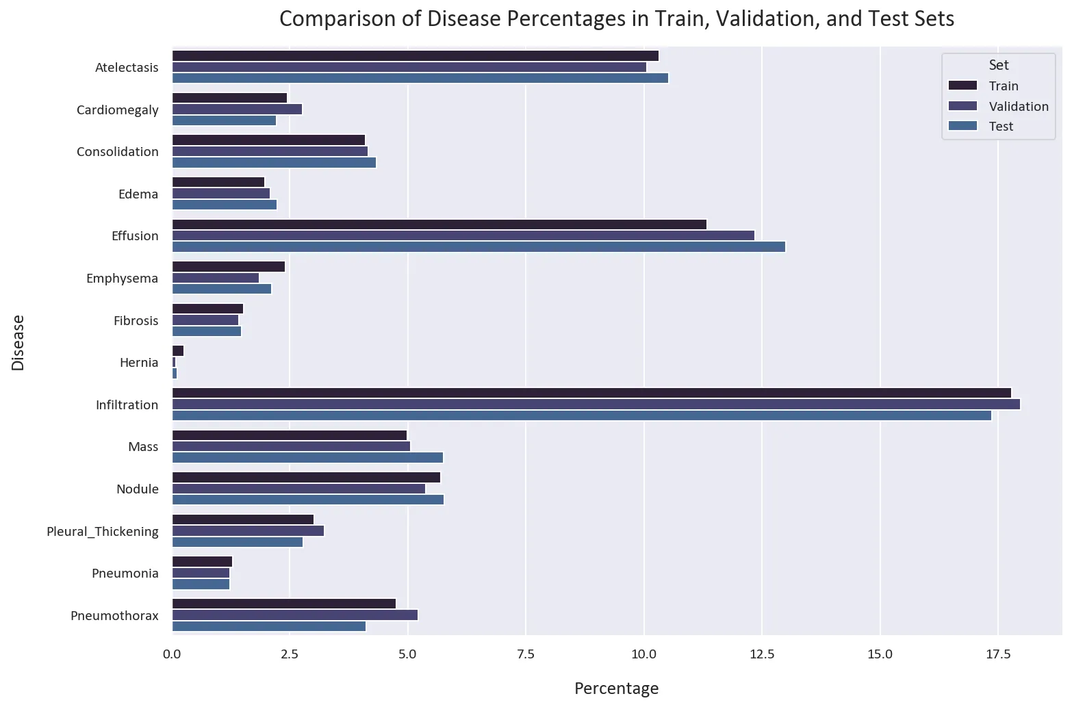
# Calculate the percentages of each disease in the train, validation, and test sets
train_percentages = train_df[diseases].mean() * 100
val_percentages = val_df[diseases].mean() * 100
test_percentages = test_df[diseases].mean() * 100

# Create a DataFrame that contains the calculated percentages
percentage_df = pd.DataFrame({
  'Disease': diseases,
  'Train': train_percentages,
  'Validation': val_percentages,
  'Test': test_percentages
})

# Melt the DataFrame from wide format to long format for plotting
percentage_df = percentage_df.melt(id_vars='Disease', var_name='Set', value_name='Percentage')

# Create a bar plot that compares the percentages of each disease in the train, validation, and test sets
plt.figure(figsize=(12, 8))
sns.barplot(data=percentage_df, x='Percentage', y='Disease', hue='Set', alpha=1)
plt.title('Comparison of Disease Percentages in Train, Validation, and Test Sets')
plt.show()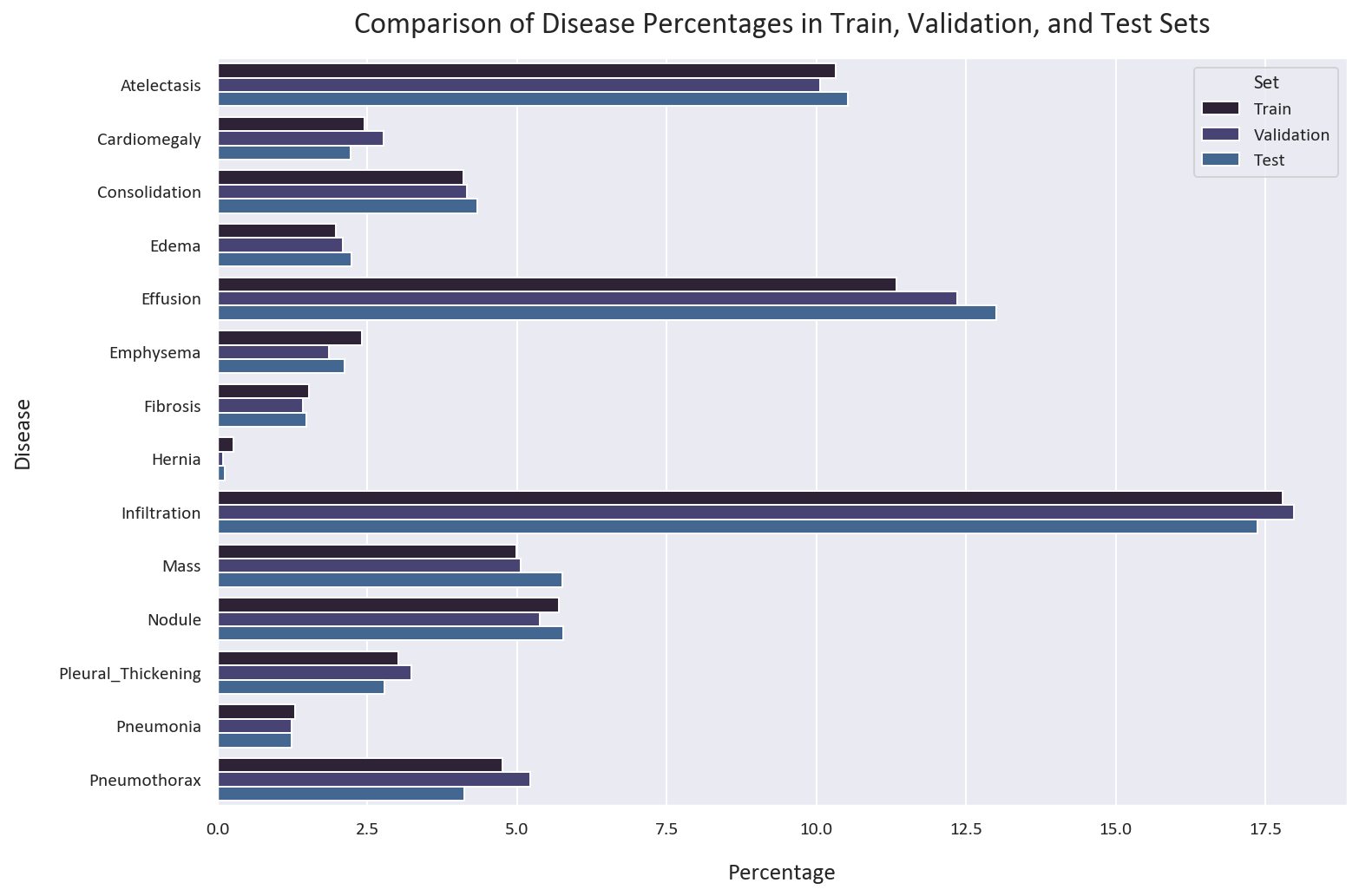

The distribution of the classes is similar in all datasets. This is good, as we want to have a similar distribution of the classes in all datasets.

Next, we want to calculate the class weights for the diseases:

class_weights = []

for i, disease in enumerate(diseases):
  # Count the number of positive and negative instances for this disease
  n_positive = np.sum(train_df[disease])
  n_negative = len(train_df) - n_positive

  # Compute the weight for positive instances and the weight for negative instances
  weight_for_positive = (1 / n_positive) * (len(train_df) / 2.0)
  weight_for_negative = (1 / n_negative) * (len(train_df) / 2.0)

  class_weights.append({0: weight_for_negative, 1: weight_for_positive})

# Now class_weights is a list of dictionaries, where each dictionary contains the weights for one disease
class_weights

Which gives us the following class weights:

[{0: 0.5575824102160178, 1: 4.841603608847497},
 {0: 0.5125868523625383, 1: 20.361995104039167},
 {0: 0.5213824552606011, 1: 12.191828508611213},
 {0: 0.5101034879264086, 1: 25.24393019726859},
 {0: 0.5639332870048644, 1: 4.410326086956522},
 {0: 0.5123973942371368, 1: 20.66552795031056},
 {0: 0.5077912762125698, 1: 32.5871694417238},
 {0: 0.5013259601910588, 1: 189.04261363636365},
 {0: 0.6081985193309569, 1: 2.810567663456665},
 {0: 0.5262562674975879, 1: 10.021536144578315},
 {0: 0.5302062085670577, 1: 8.776444209970984},
 {0: 0.5155494607660841, 1: 16.577727952167415},
 {0: 0.5065928711725566, 1: 38.41974595842956},
 {0: 0.5249775155024694, 1: 10.509001895135818}]

Here’s a step-by-step explanation of the code:

• For each disease in the diseases list, it counts the number of positive instances (n_positive) and negative instances (n_negative).

• It then calculates the weight for positive instances (weight_for_positive) and the weight for negative instances (weight_for_negative). The weight is inversely proportional to the number of instances, meaning that less frequent classes will have a higher weight. This will give more importance to under-represented classes during training. It then multiplies the weights by half of the total number of instances as there are two classes (0 and 1).

• By dividing the total number of instances (len(train_df)) by 2, we’re effectively allocating half of the total weight to the positive instances and the other half to the negative instances.

• This way, when the weights are applied during model training, the model sees as if it’s dealing with a balanced dataset, where the positive and negative classes have an equal total weight.

• It stores the weights for each class (0 and 1) in a dictionary and appends this dictionary to the class_weights list.

• The resulting class_weights list is a list of dictionaries, where each dictionary contains the weights for one disease. These weights can be used in the fit method of a Keras model via the class_weight argument to give more importance to under-represented classes during training.

Next, we’ll create a function to load and preprocess our images:

def load_image(image_path, size=IMG_SIZE):
  """
  Load the image from the given path and resize it to the given size.
  """
  # Read the image file
  image = tf.io.read_file(image_path)
  # Decode the JPEG image to a tensor
  image = tf.image.decode_jpeg(image, channels=1)  # Grayscale image
  # Resize the image
  image = tf.image.resize(image, size)
  return image

# Load the training images to calculate mean and std for standardization
train_images = np.stack([load_image(path) for path in train_df['Image Path']], axis=0)
train_mean = np.mean(train_images)
train_std = np.std(train_images)

print(f'Mean: {train_mean:.2f}')
print(f'Standard Deviation: {train_std:.2f}')

In this code, we use the mean and standard deviation of the training dataset to standardize the training, validation, and testing datasets. This is because we want to simulate the real world, where we only have the training dataset and we want to use it to standardize the validation and testing datasets.

Standardizing the images is a common preprocessing step in image processing tasks. It helps to make the model less sensitive to the scale of features, which can be particularly important for images that have pixel intensity values in different ranges.

By standardizing, we ensure that the pixel intensity values have a mean of 0 and a standard deviation of 1. This can help the model converge faster during training and can also lead to better performance, as the optimizer can more easily find a good solution in a standardized space.

Standardization also helps to ensure that the initial weights are in a good range to start with, which can prevent issues with vanishing or exploding gradients during backpropagation.

Now we’ll create our TensorFlow datasets and apply data augmentation to help with the class imbalance:

# Define the underrepresented diseases
underrepresented_diseases = ['Hernia', 'Pneumonia', 'Fibrosis', 'Emphysema', 
                         'Pleural_Thickening', 'Cardiomegaly', 'Consolidation', 
                         'Pneumothorax', 'Mass', 'Nodule']

# Define the data augmentation
data_augmentation = tf.keras.Sequential([
  tf.keras.layers.experimental.preprocessing.RandomRotation(0.1),
  tf.keras.layers.experimental.preprocessing.RandomZoom(0.2),
])

# Create base datasets
train_ds = tf.data.Dataset.from_tensor_slices((train_df['Image Path'].values, train_df[diseases].values))
train_ds = train_ds.map(lambda x, y: (load_image(x), y))
train_ds = train_ds.map(lambda x, y: ((x - train_mean) / train_std, y))

# Define augmentation function
def augment_images(image, label):
  def augment():
      return data_augmentation(image), label
  def not_augment():
      return image, label
  
  # Get indices of underrepresented diseases
  underrepresented_diseases_indices = [diseases.index(disease) for disease in underrepresented_diseases]
  
  for i in underrepresented_diseases_indices:
      condition = tf.equal(tf.gather(label, i), 1)
      image, label = tf.cond(condition, augment, not_augment)
  
  return image, label

# Create augmented dataset for underrepresented diseases
underrepresented_ds = train_ds.filter(
  lambda image, label: tf.reduce_any([tf.equal(label[i], 1) 
  for i in [diseases.index(d) for d in underrepresented_diseases]])
)
augmented_ds = underrepresented_ds.map(augment_images)

# Combine original and augmented datasets
train_ds_augmented = train_ds.concatenate(augmented_ds)
train_ds_augmented = train_ds_augmented.shuffle(1000).batch(BATCH_SIZE).prefetch(tf.data.experimental.AUTOTUNE)

# Create validation and test datasets
val_ds = tf.data.Dataset.from_tensor_slices((val_df['Image Path'].values, val_df[diseases].values))
val_ds = val_ds.map(lambda x, y: (load_image(x), y))
val_ds = val_ds.map(lambda x, y: ((x - train_mean) / train_std, y))
val_ds = val_ds.batch(BATCH_SIZE).prefetch(tf.data.experimental.AUTOTUNE)

test_ds = tf.data.Dataset.from_tensor_slices((test_df['Image Path'].values, test_df[diseases].values))
test_ds = test_ds.map(lambda x, y: (load_image(x), y))
test_ds = test_ds.map(lambda x, y: ((x - train_mean) / train_std, y))
test_ds = test_ds.batch(BATCH_SIZE).prefetch(tf.data.experimental.AUTOTUNE)

The augment_images function is designed to augment images that belong to underrepresented diseases in the dataset. Here’s a detailed breakdown:

• The function takes two arguments: image and label. The image is the input image that may be augmented, and label is the corresponding label indicating the disease.

• Two inner functions are defined: augment and not_augment. The augment function applies a data_augmentation function to the image and returns the augmented image along with its label. The not_augment function simply returns the image and label without any changes.

• The function then iterates over the indices of the underrepresented diseases (underrepresented_diseases_indices). For each index, it checks if the label at that index is 1 (indicating that the image belongs to that disease).

• The tf.equal(tf.gather(label, i), 1) operation checks if the i-th disease is present in the label. If it is (tf.equal returns True), the condition is True.

• tf.cond(condition, augment, not_augment) is a conditional operation that executes augment if the condition is True and not_augment if the condition is False.

• If the condition is True, the augment function is called, and the image is augmented. If the condition is False, the not_augment function is called, and the image is not augmented.

• The function finally returns the (possibly augmented) image and its label.

We then create datasets for the training, validation, and testing datasets using the tf.data.Dataset.from_tensor_slices function to batch and prefetch the data.

Next, we’ll create a weighted binary cross-entropy loss function to handle the class imbalance:

from keras import backend as K

def create_weighted_binary_crossentropy(class_weights):
  def weighted_binary_crossentropy(y_true, y_pred):
      # Cast the true label to float32
      y_true = tf.cast(y_true, tf.float32)
      
      # Calculate the binary cross-entropy loss
      bce = K.binary_crossentropy(y_true, y_pred)
      
      # Apply the weights for each class
      weighted_bce = 0
      for i in range(len(class_weights)):
          weights = y_true[:, i] * class_weights[i][1] + (1. - y_true[:, i]) * class_weights[i][0]
          weighted_bce += weights * bce[:, i]
          
      return K.mean(weighted_bce)
  
  return weighted_binary_crossentropy

Here’s a step-by-step explanation for the custom loss function:

1. The function create_weighted_binary_crossentropy is defined with one parameter: class_weights. This is a list of dictionaries, where each dictionary contains the weights for one disease.

2. Inside this function, another function weighted_binary_crossentropy is defined. This function calculates the weighted binary cross-entropy loss for the predictions. It takes two parameters: y_true and y_pred, which represent the true labels and the predicted labels, respectively.

3. y_true is cast to tf.float32 to ensure that the calculations are done in floating point numbers.

4. The binary cross-entropy loss bce is calculated using K.binary_crossentropy(y_true, y_pred). This function calculates the binary cross-entropy between the true labels and the predicted labels.

5. An empty variable weighted_bce is initialized to store the weighted binary cross-entropy loss.

6. A for loop is used to iterate over the range of the length of class_weights. For each class, it calculates the weights for the positive and negative instances. This is done by multiplying the true labels for the class(the positive instances) (y_true[:, i]) with the weight for the positive instances (class_weights[i][1]) and adding the result to the product of the complement of the true labels(which would be the negative instances) (1. - y_true[:, i]) and the weight for the negative instances (class_weights[i][0]).

7. The calculated weights are then multiplied with the binary cross-entropy loss for the class (bce[:, i]) and added to weighted_bce.

8. After the for loop, the function returns the mean of the weighted binary cross-entropy loss using K.mean(weighted_bce).

9. Finally, create_weighted_binary_crossentropy returns the weighted_binary_crossentropy function. This allows me to create a custom loss function with specific class weights, which I can then pass to the compile method of my model.

Now we can build our model, As this is an image classification problem, we will use a convolutional neural network (CNN):

# Define the model
model_cnn = tf.keras.Sequential([
  tf.keras.layers.Conv2D(16, (7, 7), activation='relu', input_shape=(IMG_SIZE[0], IMG_SIZE[1], 1)),
  tf.keras.layers.MaxPooling2D((2, 2)),
  tf.keras.layers.BatchNormalization(),
  
  tf.keras.layers.Conv2D(32, (7, 7), activation='relu'),
  tf.keras.layers.MaxPooling2D((2, 2)),
  tf.keras.layers.BatchNormalization(),
  
  tf.keras.layers.Conv2D(64, (7, 7), activation='relu'),
  tf.keras.layers.MaxPooling2D((2, 2)),
  tf.keras.layers.BatchNormalization(),
  
  tf.keras.layers.Conv2D(128, (7, 7), activation='relu'),
  tf.keras.layers.MaxPooling2D((2, 2)),
  tf.keras.layers.BatchNormalization(),
  
  tf.keras.layers.GlobalAveragePooling2D(),
  tf.keras.layers.Dropout(0.2),
  tf.keras.layers.Dense(len(diseases), activation='sigmoid')
])

# Define the AUC metric
AUC = tf.keras.metrics.AUC(multi_label=True, name='auc')

# Compile the model
model_cnn.compile(
  loss=create_weighted_binary_crossentropy(class_weights),
  optimizer='adam',
  metrics=['binary_accuracy', AUC, 
           tf.keras.metrics.Recall(name='recall'), 
           tf.keras.metrics.Precision(name='precision')]
)

# Print model summary
model_cnn.summary()

I used a larger kernel size of 7x7 for the first convolutional layer. This is because larger kernel sizes can be beneficial in medical imaging tasks for the following reasons:

1. Coverage: A larger kernel size means that the convolution operation covers a larger area of the input image. This can be beneficial when the important features in the image are large or spread out, which is often the case in X-ray images where the disease markers can be spread across the image.

2. Context: Larger kernels can capture more context. In medical imaging, the context around a certain area can provide important information about the presence or absence of a disease.

3. Noise Reduction: Larger kernels can also act as a noise reduction mechanism, as they average more pixels together. This can be beneficial in medical imaging, where images can often contain noise.

However, it’s important to note that larger kernels come with their own trade-offs. They are more computationally expensive and may miss finer details that smaller kernels could capture. Therefore, the choice of kernel size should be based on the specific task and nature of the input data, and often involves a process of experimentation and validation. I found that a kernel size of 7x7 worked well for this task.

Let’s train our model:

# Define the number of epochs
EPOCHS = 20

# Train the model
history_cnn = model_cnn.fit(
  train_ds_augmented,
  validation_data=val_ds,
  epochs=EPOCHS,
  callbacks=[
      tf.keras.callbacks.EarlyStopping(
          patience=5, 
          monitor='val_loss', 
          restore_best_weights=True
      ),
      tf.keras.callbacks.ModelCheckpoint(
          'models/model-weighted-binary-crossentropy.keras',
          monitor='val_loss',
          save_best_only=True,
          verbose=1
      ),
      tf.keras.callbacks.LearningRateScheduler(
          lambda epoch: 1e-3 * 0.95 ** epoch,
          verbose=1
      )
  ]
)

In the code above, I used a learning rate scheduler to help the model converge faster, which multiplied the learning rate by 0.95 for each epoch. I also used an early stopping callback to stop the training if the validation loss doesn’t improve for 5 epochs and a model checkpoint callback to save the best model.

Model Evaluation and Comparison

Let’s evaluate our model’s training history:

plt.figure(figsize=(12, 8))
plt.subplot(2, 2, 1)
plt.plot(history_cnn.history['loss'], label='Training Loss')
plt.plot(history_cnn.history['val_loss'], label='Validation Loss')
plt.legend()
plt.xlabel('Epoch')
plt.ylabel('Loss')
plt.title('Training and Validation Losses')

plt.subplot(2, 2, 2)
plt.plot(history_cnn.history['binary_accuracy'], label='Training Accuracy')
plt.plot(history_cnn.history['val_binary_accuracy'], label='Validation Accuracy')
plt.legend()
plt.xlabel('Epoch')
plt.ylabel('Accuracy')
plt.title('Training and Validation Accuracies')

plt.subplot(2, 2, 3)
plt.plot(history_cnn.history['precision'], label='Training Precision')
plt.plot(history_cnn.history['val_precision'], label='Validation Precision')
plt.legend()
plt.xlabel('Epoch')
plt.ylabel('Precision')
plt.title('Training and Validation Precisions')

plt.subplot(2, 2, 4)
plt.plot(history_cnn.history['recall'], label='Training Recall')
plt.plot(history_cnn.history['val_recall'], label='Validation Recall')
plt.legend()
plt.xlabel('Epoch')
plt.ylabel('Recall')
plt.title('Training and Validation Recalls')
plt.tight_layout()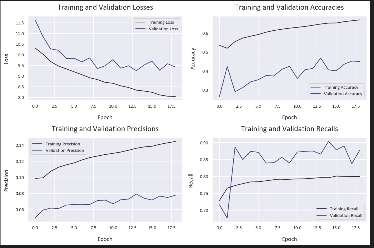

Now let’s compare our weighted binary cross-entropy model with a standard binary cross-entropy model to understand the impact of our loss function:

# Compile the model using binary cross-entropy loss
model_cnn.compile(
  loss='binary_crossentropy',
  optimizer='adam',
  metrics=['binary_accuracy', AUC, 
           tf.keras.metrics.Recall(name='recall'), 
           tf.keras.metrics.Precision(name='precision')]
)

# Train the model
history_cnn_2 = model_cnn.fit(
  train_ds_augmented,
  validation_data=val_ds,
  epochs=EPOCHS,
  callbacks=[
      tf.keras.callbacks.EarlyStopping(
          patience=5, 
          monitor='val_loss', 
          restore_best_weights=True
      ),
      tf.keras.callbacks.ModelCheckpoint(
          'models/model-binary-crossentropy.keras',
          monitor='val_loss',
          save_best_only=True,
          verbose=1
      ),
      tf.keras.callbacks.LearningRateScheduler(
          lambda epoch: 1e-3 * 0.95 ** epoch,
          verbose=1
      )
  ]
)

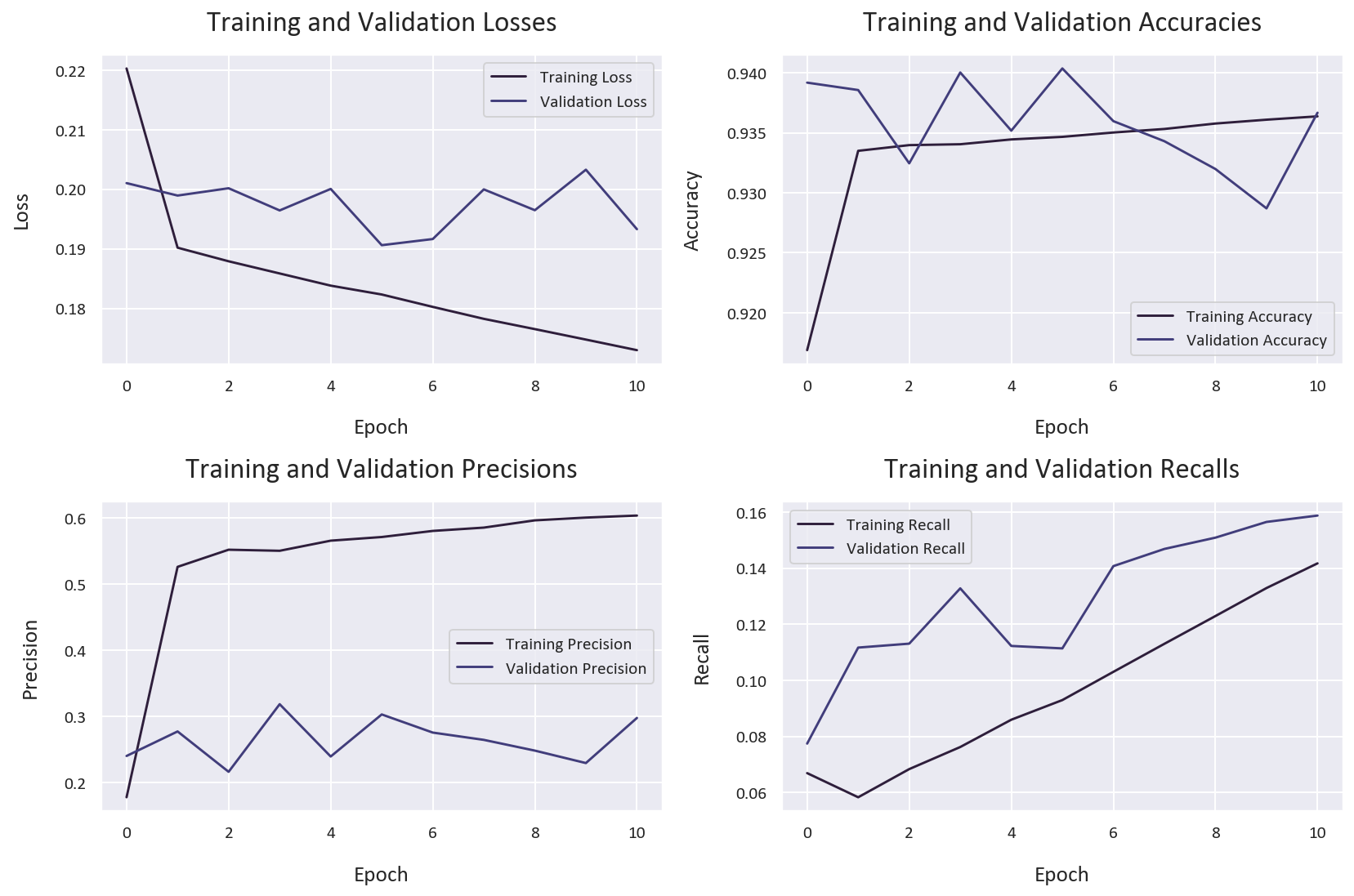
This is the training history for the standard binary cross-entropy model:

Let’s analyze the ROC curves for both models:

from sklearn.metrics import roc_curve, auc

# Load the best models
model_wbce = tf.keras.models.load_model(
  'models/model-weighted-binary-crossentropy.keras',
  custom_objects={'weighted_binary_crossentropy': create_weighted_binary_crossentropy(class_weights)}
)
model_bce = tf.keras.models.load_model('models/model-binary-crossentropy.keras')

# Get predictions
predictions_wbce = model_wbce.predict(test_ds)
predictions_bce = model_bce.predict(test_ds)

# Initialize dictionaries for both models
fpr_dict_wbce = {}
tpr_dict_wbce = {}
auc_dict_wbce = {}
fpr_dict_bce = {}
tpr_dict_bce = {}
auc_dict_bce = {}

# Compute ROC curves and AUC scores
for i, disease in enumerate(diseases):
  # Weighted Binary Cross-Entropy
  fpr, tpr, _ = roc_curve(test_df[disease], predictions_wbce[:, i])
  auc_score = auc(fpr, tpr)
  fpr_dict_wbce[disease] = fpr
  tpr_dict_wbce[disease] = tpr
  auc_dict_wbce[disease] = auc_score
  
  # Binary Cross-Entropy
  fpr, tpr, _ = roc_curve(test_df[disease], predictions_bce[:, i])
  auc_score = auc(fpr, tpr)
  fpr_dict_bce[disease] = fpr
  tpr_dict_bce[disease] = tpr
  auc_dict_bce[disease] = auc_score

# Plot ROC curves
plt.figure(figsize=(12, 8))
for disease in diseases:
  plt.plot(fpr_dict_wbce[disease], tpr_dict_wbce[disease], 
           label=f'WBCE - {disease} (AUC = {auc_dict_wbce[disease]:.2f})')
plt.plot([0, 1], [0, 1], 'k--')
plt.xlabel('False Positive Rate')
plt.ylabel('True Positive Rate')
plt.title('ROC Curves - Weighted Binary Cross-Entropy')
plt.legend(bbox_to_anchor=(1.05, 1), loc='upper left')
plt.tight_layout()
plt.show()

plt.figure(figsize=(12, 8))
for disease in diseases:
  plt.plot(fpr_dict_bce[disease], tpr_dict_bce[disease], 
           label=f'BCE - {disease} (AUC = {auc_dict_bce[disease]:.2f})')
plt.plot([0, 1], [0, 1], 'k--')
plt.xlabel('False Positive Rate')
plt.ylabel('True Positive Rate')
plt.title('ROC Curves - Binary Cross-Entropy')
plt.legend(bbox_to_anchor=(1.05, 1), loc='upper left')
plt.tight_layout()
plt.show()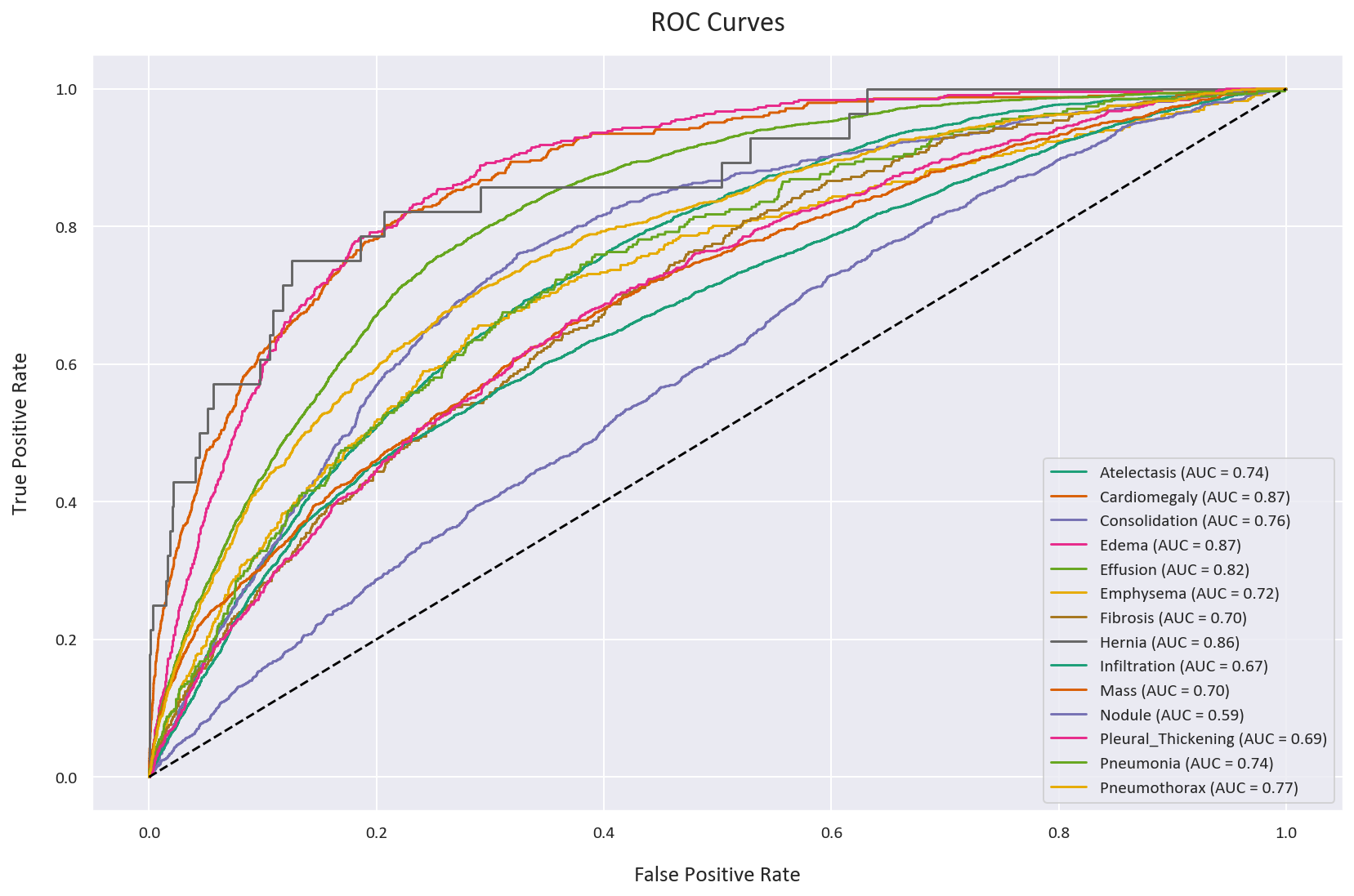

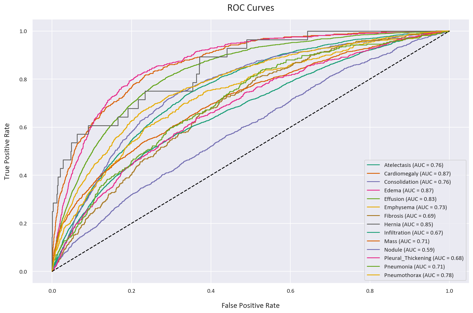
As we can see, the two ROC curves are very similar, which as discussed before, can be deceptive. They both have an AUC score of 0.75, but as we will see later, this is misleading.

Let’s compare the classification reports for both models:

from sklearn.metrics import classification_report

print('Weighted Binary Cross-Entropy Model:')
print(classification_report(
  test_df[diseases], 
  predictions_wbce > 0.5,
  target_names=diseases
))

print('
Binary Cross-Entropy Model:')
print(classification_report(
  test_df[diseases],
  predictions_bce > 0.5,
  target_names=diseases
))

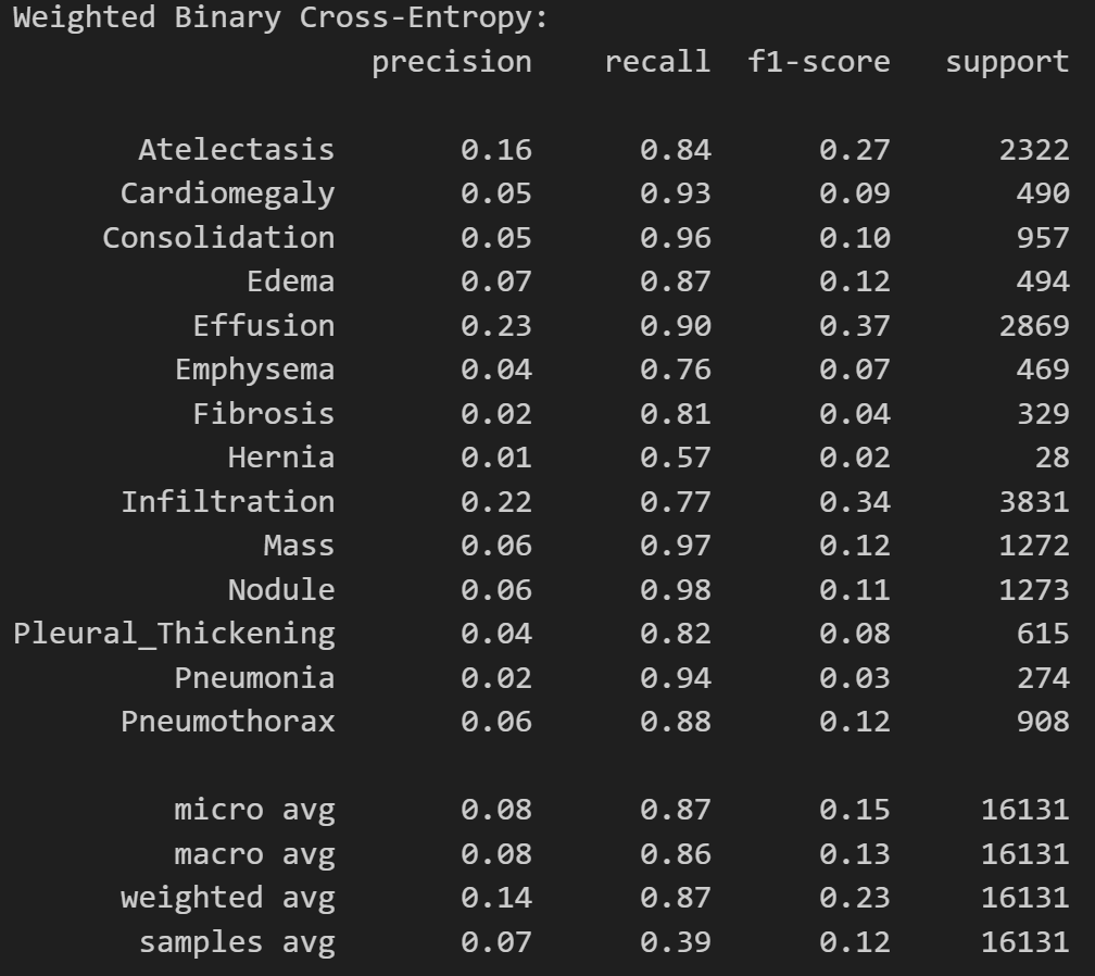
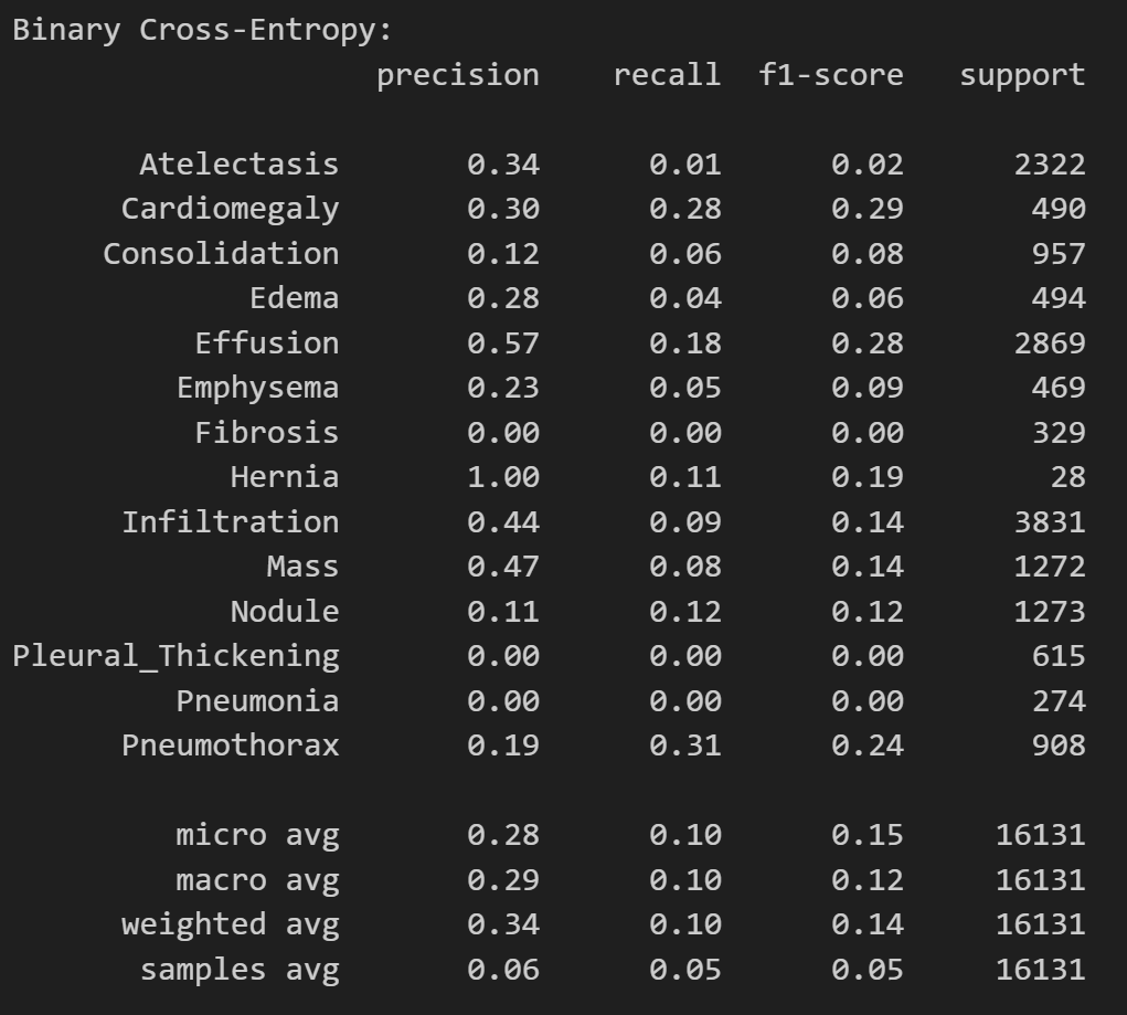
As expected, the binary cross-entropy loss model has a higher precision but abyssmal recall. This means that the model will tend to classify most patients as healthy, even if they have a disease. The weighted binary cross-entropy loss model has a lower precision but a much higher recall. This means that the model will not miss a positive sample very often. This will prevent false negatives. Which model should we use in a medical setting? Let’s find out.

Let’s further confirm this by looking at the percentage of the positive and negative cases that were correctly classified by each model.

def calculate_detection_rates(predictions, test_df, diseases):
  correctly_identified_p = {}
  correctly_identified_n = {}
  
  for disease in diseases:
      # Positive cases
      indices = test_df[test_df[disease] == 1].index
      disease_predictions = predictions[indices, diseases.index(disease)]
      correctly_identified_p[disease] = np.where(disease_predictions > 0.5)[0]
      
      # Negative cases
      indices = test_df[test_df[disease] == 0].index
      disease_predictions = predictions[indices, diseases.index(disease)]
      correctly_identified_n[disease] = np.where(disease_predictions < 0.5)[0]
  
  return correctly_identified_p, correctly_identified_n

# Calculate rates for both models
p_wbce, n_wbce = calculate_detection_rates(predictions_wbce, test_df, diseases)
p_bce, n_bce = calculate_detection_rates(predictions_bce, test_df, diseases)

# Print results for weighted binary cross-entropy model
print('Weighted Binary Cross-Entropy Model:')
print('Correctly identified positive cases:')
for disease in diseases:
  percentage = len(p_wbce[disease]) / len(test_df[test_df[disease] == 1]) * 100
  print(f'{disease}: {percentage:.2f}%')

print('
Correctly identified negative cases:')
for disease in diseases:
  percentage = len(n_wbce[disease]) / len(test_df[test_df[disease] == 0]) * 100
  print(f'{disease}: {percentage:.2f}%')

# Print results for binary cross-entropy model
print('
Binary Cross-Entropy Model:')
print('Correctly identified positive cases:')
for disease in diseases:
  percentage = len(p_bce[disease]) / len(test_df[test_df[disease] == 1]) * 100
  print(f'{disease}: {percentage:.2f}%')

print('
Correctly identified negative cases:')
for disease in diseases:
  percentage = len(n_bce[disease]) / len(test_df[test_df[disease] == 0]) * 100
  print(f'{disease}: {percentage:.2f}%')

These are the percentages:

Weighted Binary Cross-Entropy:
Total percentage of correctly identified positive cases for all diseases: 86.62%
Total percentage of correctly identified negative cases for all diseases: 44.84%

Binary Cross-Entropy:
Total percentage of correctly identified positive cases for all diseases: 10.31%
Total percentage of correctly identified negative cases for all diseases: 98.54%

Conclusion

As we suspected earlier, the binary cross-entropy loss model has a high accuracy because it classifies most cases as negative. This is why it has a high precision but a low recall. This lead to it identifying 98.54% of the negative cases correctly but only 10.31% of the positive cases correctly. This is extremely dangerous.

The weighted binary cross-entropy loss model can distinguish between the positive and negative cases much better. This is why it has a lower accuracy but a higher recall. This lead to it identifying 86.62% of positive cases correctly and 44.84% of the negative cases correctly.

This is much, much better than the binary cross-entropy loss model. Yes, 55.16% of healthy patients were misdiagnosed, but patients usually go for further testing to confirm the diagnosis. This is contrary to patients with a disease, where if they were told they do not have a disease, they may not go for further testing until the symptoms get worse. This is usually too late and can make recovery much harder. This is why we want to minimize the number of false negatives, even if it means increasing the number of false positives.

This project demonstrates the importance of carefully considering evaluation metrics and loss functions in medical imaging applications, where the cost of false negatives can be much higher than false positives.

You can find the code for this project here .